01 Liquidity Mathematical Expressions

Overview

In the overview of the Uniswap V3 protocol, we understood the core ideas of V3 from a macro perspective, including:

• Liquidity is no longer distributed across the price range $(0, \infty)$
• but concentrated in a limited interval $[p_{\text{lower}}, p_{\text{upper}}]$
• By introducing virtual liquidity, the local curve still satisfies the constant product relationship

$$(x_R + x_V)(y_R + y_V) = L^2$$

However, this expression remains static. During real trading, prices continue to change, so how does liquidity affect prices? How does the quantity of an asset change with price? These questions require a more precise mathematical description.

This chapter starts from the perspective of Liquidity and systematically answers the following key questions:

1. Asset status at different price positions

When the price $P$ is in different ranges:

• $P < p_{\text{lower}}$: holds only token0
• $p_{\text{lower}} < P < p_{\text{upper}}$: holds both assets
• $P > p_{\text{upper}}$: holds only token1

We will derive in different states:

$$x_R(P), \quad y_R(P)$$

2. Global liquidity and interval liquidity

• global liquidity (effective liquidity at the current price)
• liquidity net (change across ticks)

Understand why liquidity is "segmented".

3. Virtual reserves and real reserves

• How to calculate $x_V, y_V$ (virtual assets)
• How to calculate $x_R, y_R$ (real assets)
• What they mean in different price ranges

4. Calculation of liquidity $L$

• How to calculate $L$ based on the number of tokens
• How to deduce the number of tokens based on $L$
• The relationship between $L$ and price

Through this chapter, we will establish a complete understanding that price changes in Uniswap V3 are essentially driven by liquidity. These formulas will be used repeatedly as the basis for later analysis of ticks, swaps, fee calculation, and other mechanisms.

1. Asset status at different price positions

In Uniswap V3, the liquidity provided by an LP only takes effect within the interval $[p_{\text{lower}}, p_{\text{upper}}]$. As the price $P$ changes, the asset structure held by the LP changes as well.

1.1 When $P > p_{\text{upper}}$ (price is above the range)

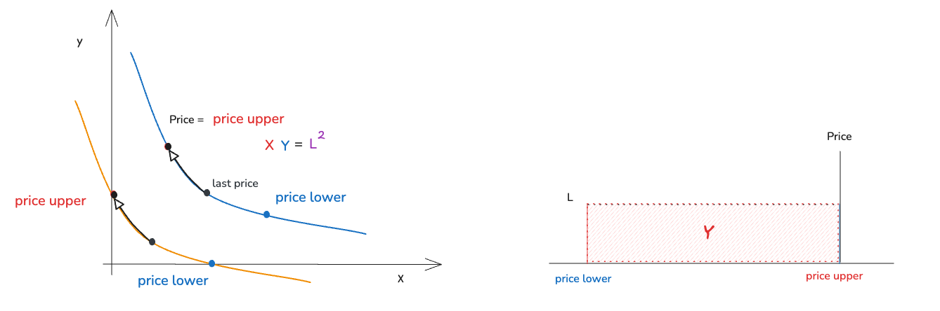
At this point, the price has completely crossed the LP range.

It can be observed:

• All liquidity is represented as token1(Y)
• token0(X) is 0

Right now:

$$x_R = 0, \quad y_R > 0$$

The LP's token0 has been fully sold and replaced by token1.

1.2 When $P < p_{\text{lower}}$ (price is below the range)

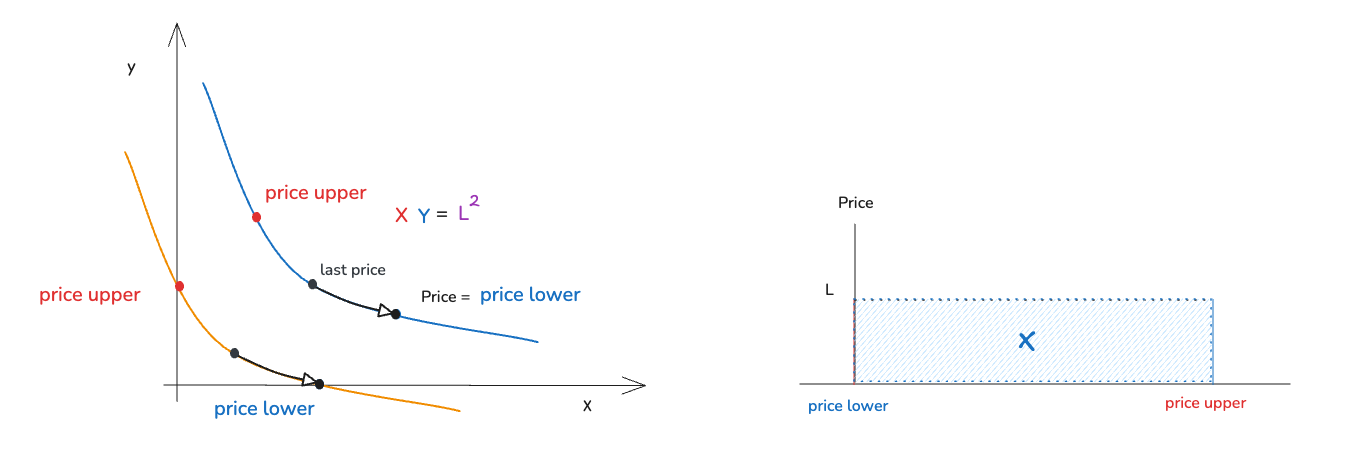
At this time, the price leaves the LP's market-making range.

It can be observed:

• All liquidity is represented as token0(X)
• token1(Y) is 0

Right now:

$$x_R > 0, \quad y_R = 0$$

From the curve's point of view, the state point stays at the left boundary of the interval. What the LP provides is token0 waiting to be bought.

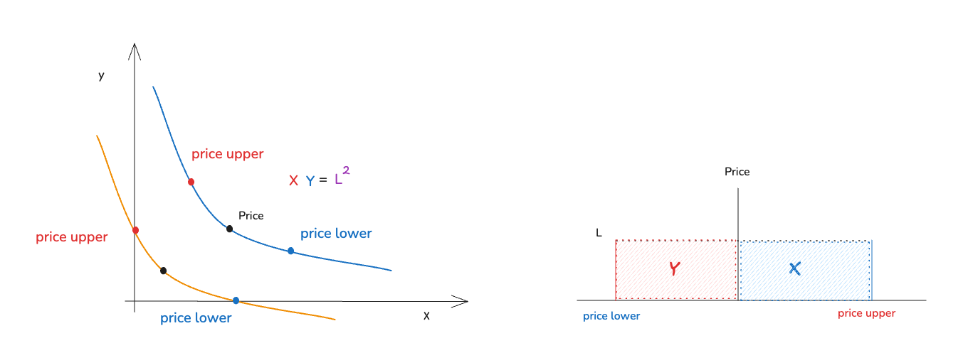
1.3 When $p_{\text{lower}} < P < p_{\text{upper}}$ (price is within the range)

At this point, liquidity is active.

As the price moves:

• token0(X) gradually decreases
• token1(Y) gradually increases

Right now:

$$x_R > 0, \quad y_R > 0$$

and satisfies:

$$(x_R + x_V)(y_R + y_V) = L^2$$

The liquidity status can be summarized into three segments:

$$\begin{cases} P < p_{\text{lower}} & \Rightarrow (x_R > 0, \; y_R = 0) \\ p_{\text{lower}} < P < p_{\text{upper}} & \Rightarrow (x_R > 0, \; y_R > 0) \\ P > p_{\text{upper}} & \Rightarrow (x_R = 0, \; y_R > 0) \end{cases}$$

Liquidity is not "providing two assets at the same time", but constantly switching between token0 and token1 as the price changes. Price movement is essentially the redistribution of LP assets between X and Y.

2. Global liquidity and interval liquidity

In Uniswap V3, each LP position only provides liquidity within the interval $[p_{\text{lower}}, p_{\text{upper}}]$. However, Pool does not calculate the current liquidity position by position, but maintains a global state:

$$L = \text{current active liquidity}$$

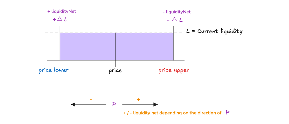
At each price (actually it should be represented by tick, here price is used for ease of understanding), the protocol does not store the complete liquidity distribution, but records a key variable liquidityNet. It represents the net change in global liquidity when the price crosses the price (tick).

When the price $P$ changes, the Pool will update the liquidity according to the direction of price movement:

2.1 When the price moves to the right (increases):

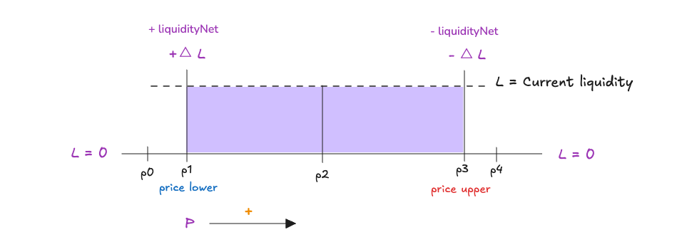
• $p0$ liquidity is the initial value, $L = 0$
• $p1$ When price enters the range $[p_{\text{lower}}, p_{\text{upper}}]$, start adding liquidityNet, $L + \Delta L = 0 + \Delta L = \Delta L$
• $p2$ When the price continues to rise, it moves right to the middle. The current liquidity is still $\Delta L$ stored in the range.
• $p3$ When the price rises to the $p_{\text{upper}}$ boundary, it has left the range. liquidity reduces liquidity within the range, $L = 0$

2.2 When the price moves to the left (falls):

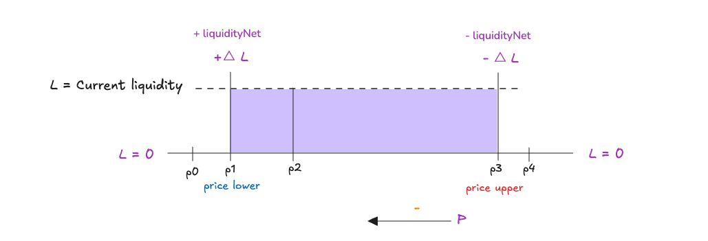
• $p4$ liquidity is the initial value, $L = 0$
• $p3$ When price enters the range $[p_{\text{lower}}, p_{\text{upper}}]$, start adding liquidityNet, $L + \Delta L = 0 -(-\Delta L) = \Delta L$
• $p2$ When the price continues to fall, move left to the middle, and the current liquidity is still $\Delta L$ stored in the range.
• $p0$ When the price drops to the $p_{\text{lower}}$ boundary, it has left the range. liquidity reduces liquidity within the range, $L = 0$

2.3 Superposition of interval liquidity

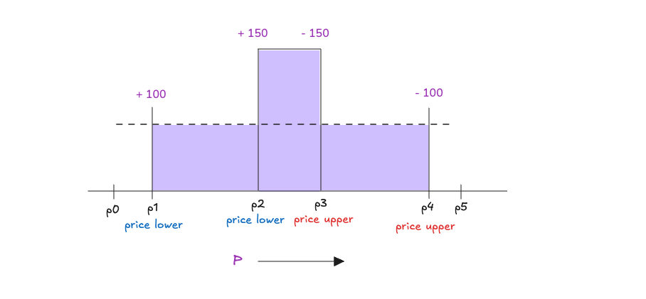
If multiple LP positions are placed on the same price axis, the liquidity distribution as shown in the figure can be obtained.

When multiple positions overlap:

• Within the same price range, liquidity will accumulate

• At borders, liquidity jumps

• $p_0:$ liquidity is initialized as $L = 0$

• $p_1:$ the price increases and enters the first interval, liquidity starts to add liquidityNet:

  $L = 0 + 100 = 100$

• $p_2:$ the price continues to move right and enters the second interval, liquidity keeps adding liquidityNet:

  $L = 100 + 150 = 250$

• $p_3:$ the price leaves the second interval, liquidity removes the corresponding liquidityNet:

  $L = 250 - 150 = 100$

• $p_4:$ the price leaves the first interval, liquidity removes the corresponding liquidityNet:

  $L = 100 - 100 = 0$

• $p_5:$ liquidity leaves all intervals, and the price moves to an uninitialized region, so liquidity remains 0

Therefore, liquidity is determined by a set of liquidityNet distributed over price (tick). When the price $P$ changes, the behavior of the Pool can be abstracted as scanning along the price direction on the tick axis and applying liquidityNet one by one.

Therefore, global liquidity can be expressed as:

$$L(P) = \sum_{\text{ticks crossed}} liquidityNet$$

3. Virtual reserves and real reserves

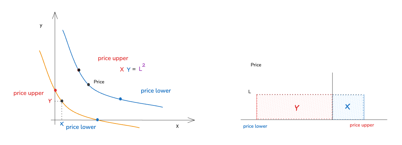
3.1 Virtual Reserve

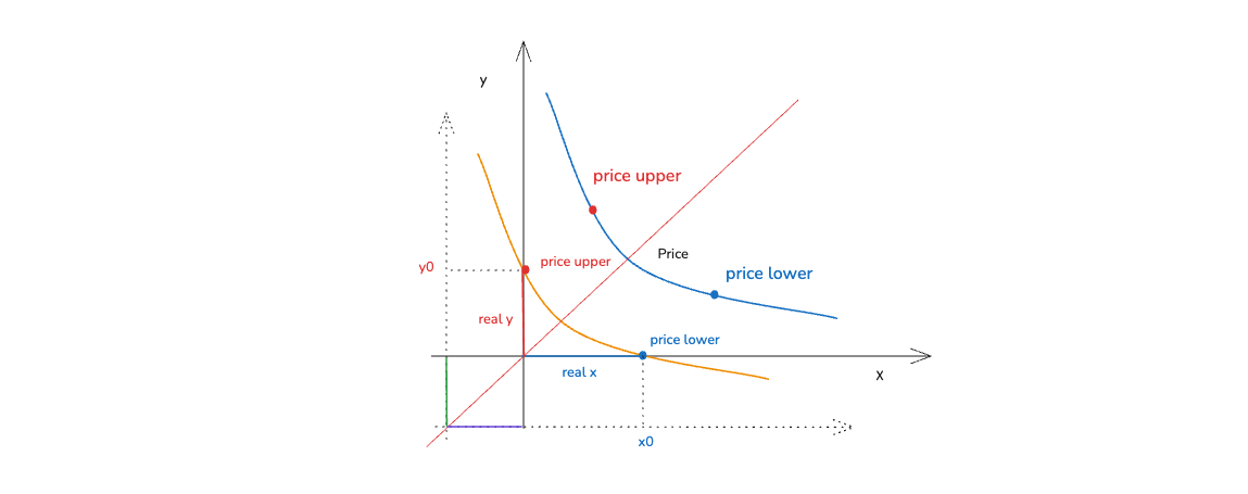
In V3, interval liquidity is no longer globally distributed, but concentrated within a limited interval. But this curve itself does not exist independently, but is embedded in a more complete AMM curve. To still maintain a continuous and consistent price function, V3 introduces virtual liquidity. Its essence is to introduce an offset x_virtual, y_virtual in the x and y directions to embed the current true state (x, y) into a larger coordinate system, so that the state still falls on a complete AMM curve.

In the picture we can see:

• $x_0$: When the price is at $P_{\text{lower}}$ (lower bound), the total real token0 quantity of this position

• $y_0$: When the price is at $P_{\text{upper}}$ (upper bound), the total real token1 quantity of this position

• virtual x is the quantity of token 0

• virtual y is the quantity of token 1

Therefore, when the price is within the range, the real reserve of $X$ is greater than 0 and less than $x_0$ (if it is greater than $x_0$, it is another range) In the same way, the real reserve of $Y$ is also greater than 0 and less than $y_0$ (if it is greater than $y_0$, it is another range)

It should be noted that $x_V$ and $y_V$ are not arbitrarily introduced offsets. The reason why they can be uniquely determined is that they themselves still belong to the coordinate quantities on the complete constant product curve. In order for the current real state $(x_R, y_R)$ to still fall on a complete constant product curve, we require:

$$(x_R + x_V)(y_R + y_V) = L^2$$

Among them, $x_V, y_V$ is the virtual reserve that needs to be solved.

Step 1: Write the coordinate relationship on the complete curve

For the complete curve:

$$XY = L^2$$

Price is defined as:

$$P = \frac{Y}{X}$$

Available together:

$$X = \frac{L}{\sqrt{P}}, \qquad Y = L\sqrt{P}$$

Simplify the process:

$$\frac{L^2}{P} = \frac{XY}{\frac{Y}{X}} = X^2 => X = \frac{L}{\sqrt{P}}$$

$$L^2 P = XY \cdot \frac{Y}{X} = Y^2 => Y = L\sqrt{P}$$

This means that when the price is $P$, the horizontal and vertical coordinates on the complete curve can be expressed as the above formulas respectively.

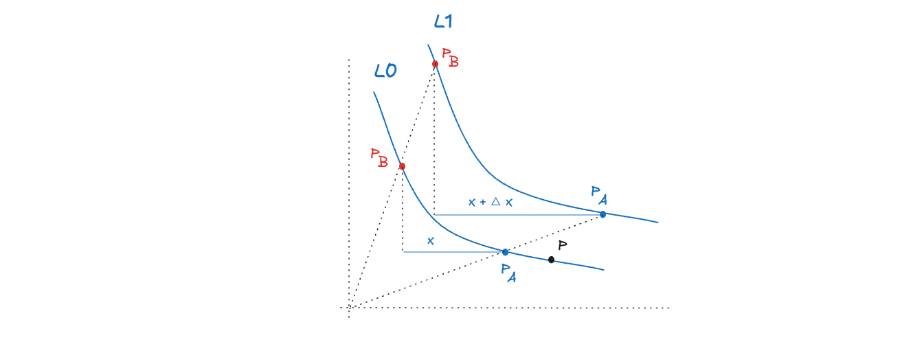
Step 2: Use boundary conditions to find $x_V$ ($P_B$ will be used to represent P upper, and $P_A$ will be used to represent $P_{\text{lower}}$)

When the price reaches the upper bound $P_{\text{upper}}$, the position has been completely converted into token1, therefore:

$$x_R = 0$$

At this time, the abscissa on the complete curve consists only of the virtual part, so:

$$x_V(y_R + y_V) = L^2$$

$$x_V = \frac {L^2}{y_R + y_V}$$

$$x_V = \frac{L^2}{L\sqrt{P_B}}$$

$$x_V = \frac{L}{\sqrt{P_B}}$$

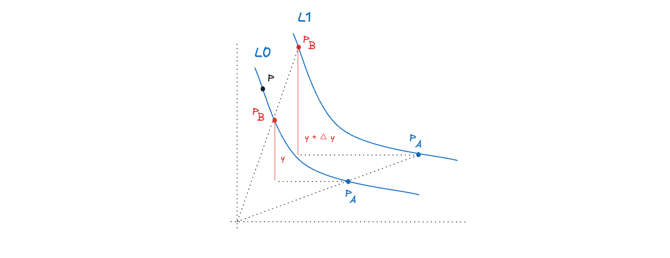
Step 3: Use boundary conditions to find $y_V$

When the price reaches the lower bound $P_{\text{lower}}$, the position has been completely converted to token0, therefore:

$$y_R = 0$$

At this time, the ordinate on the complete curve consists only of the virtual part, so:

$$(x_R+x_V)y_V = L^2$$

$$y_V = \frac{L^2}{x_R+x_V}$$

$$y_V = \frac{L^2}{\frac{L}{\sqrt{P_A}}}$$

$$y_V = L\sqrt{P_A}$$

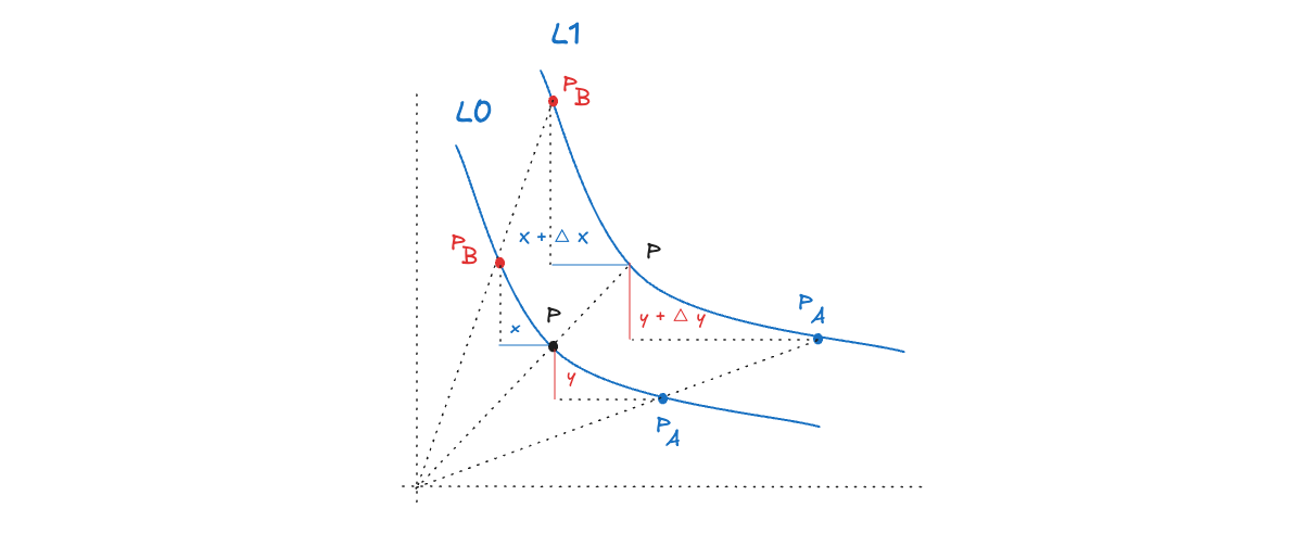
Step 4: Substitute $x_V, y_V$ into the main equation to get:

$$\left(x_R + \frac{L}{\sqrt{P_B}}\right)\left(y_R + L\sqrt{P_A}\right)=L^2$$

This is the core relationship between real reserves and virtual reserves in Uniswap V3.

3.2 Real Reserve

In the previous section, we embedded the current state $(x_R, y_R)$ into the full curve by introducing a virtual reserve:

$$(x_R + x_V)(y_R + y_V) = L^2$$

And find:

$$x_V = \frac{L}{\sqrt{P_B}}, \qquad y_V = L\sqrt{P_A}$$

When price moves within a range:

• Price increase ($P_{\text{lower}} \rightarrow P_{\text{upper}}$):
• token0 is constantly being sold
• token1 keeps increasing
• Eventually becomes pure $y_0$ (i.e. $x_0 = 0$)

$$\left( 0 + \frac{L}{\sqrt{P_B}} \right) \left( {y_0} + L \sqrt{P_A} \right) = L^2$$

Simplify:

$$\frac{L}{\sqrt{P_B}} \left( y_0 + L \sqrt{P_A} \right) = L^2$$

$$y_0 + L \sqrt{P_A} = L \sqrt{P_B}$$

Finally got:

$$y_0 = L\sqrt{P} - L\sqrt{P_A}$$

• Price decrease ($P_{\text{upper}} \rightarrow P_{\text{lower}}$):
• token1 is constantly being sold
• token0 keeps increasing
• Eventually becomes pure $x_0$ (i.e. $y_0 = 0$)

$$\left( x_0 + \frac{L}{\sqrt{P_B}} \right) \left( {0} + L \sqrt{P_A} \right) = L^2$$

Simplify:

$$\left( x_0 + \frac{L}{\sqrt{P_B}} \right)\sqrt{P_A} = L^2$$

$$x_0 + \frac{L}{\sqrt{P_B}} = \frac{L}{\sqrt{P_A}}$$

Finally got:

$$x_0 = \frac{L}{\sqrt{P}} - \frac{L}{\sqrt{P_B}}$$

Therefore, $x_0$ and $y_0$ are the "limit asset states" of this position at both ends of the range. More importantly, they provide the boundary conditions that connect the current state $(x_R, y_R)$ to the price range.

Summarize

• virtual reserves: used to construct a complete curve
• real reserves: are the assets actually held at the current price

The relationship between the two:

$$\text{real} = \text{global curve} - \text{virtual offset}$$

This is also the core way Uniswap V3 embeds “local liquidity” into “global AMM”.

4. Calculation of liquidity $L$

In the previous section we already got the real reserves:

$$x_R = \frac{L}{\sqrt{P}} - \frac{L}{\sqrt{P_B}}, \qquad y_R = L\sqrt{P} - L\sqrt{P_A}$$

This shows that in Uniswap V3, the number of tokens is not stored directly, but is determined by $L$ and the price.

Therefore, we can do two things:

• Given the number of tokens, infer $L$
• Given $L$, calculate the number of tokens

The two are essentially different variations of the same set of formulas.

4.1 Liquidity calculated by the number of Tokens

It is known that the user wants to provide in the interval $[P_{\text{lower}}, P_{\text{upper}}]$:

• $x$（token0）
• $y$（token1）

The current price is $P_c$

---

Case 1: $P_c < P_A$ (price below range)

At this point position is completely token0:

$$L = x \cdot \frac{\sqrt{P_A} \cdot \sqrt{P_B}}{\sqrt{P_B} - \sqrt{P_A}}$$

---

Case 2: $P_A \le P_c < P_B$ (price is within the range)

At this time, both token0 and token1 are held.

Use two tokens to derive liquidity:

$$L_0 = x \cdot \frac{\sqrt{P_c} \cdot \sqrt{P_B}}{\sqrt{P_B} - \sqrt{P_c}}$$

$$L_1 = \frac{y}{\sqrt{P_c} - \sqrt{P_A}}$$

Finally, take the smaller value (to ensure that both tokens can be satisfied):

$$L = \min(L_0, L_1)$$

---

Case 3: $P_c \ge P_B$ (price is higher than the range)

At this point position is entirely token1:

$$L = \frac{y}{\sqrt{P_B} - \sqrt{P_A}}$$

4.2 Calculate the number of Tokens by Liquidity

Known:

• $L$
• $P_A, P_B$
• Current price $P_c$

Calculate first:

$$\sqrt{P_c}, \quad \sqrt{P_A}, \quad \sqrt{P_B}$$

---

Case 1: $P_c < P_A$

The position consists entirely of token0:

$$\text{amount}_0 = L \cdot \left(\frac{1}{\sqrt{P_A}} - \frac{1}{\sqrt{P_B}}\right)$$

$$\text{amount}_1 = 0$$

---

Case 2: $P_A \le P_c < P_B$

Hold two tokens at the same time:

$$\text{amount}_0 = L \cdot \left(\frac{1}{\sqrt{P_c}} - \frac{1}{\sqrt{P_B}}\right)$$

$$\text{amount}_1 = L \cdot \left(\sqrt{P_c} - \sqrt{P_A}\right)$$

---

Case 3: $P_c \ge P_B$

The position consists entirely of token1:

$$\text{amount}_0 = 0$$

$$\text{amount}_1 = L \cdot \left(\sqrt{P_B} - \sqrt{P_A}\right)$$

---

As mentioned at the beginning of this section, in the previous article we have already obtained:

$$x_R = \frac{L}{\sqrt{P}} - \frac{L}{\sqrt{P_B}}, \qquad y_R = L\sqrt{P} - L\sqrt{P_A}$$

You can see:

• $\text{amount}_0$ is essentially $x_R$
• $\text{amount}_1$ is essentially $y_R$

The Token quantity formula is the expansion of the real reserve formula in different price ranges.

• virtual reserves: defines the location of the complete curve
• real reserves: Define the tokens currently held
• liquidity $L$: defines the "scale" of the curve

The relationship between the three:

$$(x_R + x_V)(y_R + y_V) = L^2$$

The token calculation formula is just the specific manifestation of this relationship in different price ranges.

5. The relationship between liquidity changes and Token ($ΔL$)

• $L_0 = Liquidity before$
• $L_1 = Liquidity after$
• $\Delta L = L_1 - L_0$

---

Case 1: $P_c \le P_A$

At this time, position is completely composed of token0. When token0 ($Δx$) is added, the corresponding liquidity change is:

$$L_0 = \frac{x}{\frac{1}{\sqrt{P_A}} - \frac{1}{\sqrt{P_B}}}$$

$$L_1 = \frac{x + \Delta x}{\frac{1}{\sqrt{P_A}} - \frac{1}{\sqrt{P_B}}}$$

$$\Delta L = L_1 - L_0 = \frac{\Delta x}{\frac{1}{\sqrt{P_A}} - \frac{1}{\sqrt{P_B}}}$$

When the price is below the range:

• Only token0 is needed to provide liquidity
• Changes in liquidity are completely determined by Δx

---

Case 2: $P_c \ge P_B$

At this time, the position is completely composed of token1.

$$L_0 = \frac{y}{\sqrt{P_B} - \sqrt{P_A}}$$

$$L_1 = \frac{y + \Delta y}{\sqrt{P_B} - \sqrt{P_A}}$$

$$\Delta L = L_1 - L_0 = \frac{\Delta y}{\sqrt{P_B} - \sqrt{P_A}}$$

When the price is above the range:

• Only token1 is needed to provide liquidity
• Changes in liquidity are entirely determined by Δy

---

Case 3: $P_A < P < P_B$

At this time both token0 and token1 participate:

$$\begin{aligned} L_0 &= \frac{x}{\frac{1}{\sqrt{P}} - \frac{1}{\sqrt{P_B}}} \\ &= \frac{y}{\sqrt{P} - \sqrt{P_A}} \end{aligned}$$

$$\begin{aligned} L_1 &= \frac{x + \Delta x}{\frac{1}{\sqrt{P}} - \frac{1}{\sqrt{P_B}}} \\ &= \frac{y + \Delta y}{\sqrt{P} - \sqrt{P_A}} \end{aligned}$$

$$\begin{aligned} \Delta L &= L_1 - L_0 \\ &= \frac{\Delta x}{\frac{1}{\sqrt{P}} - \frac{1}{\sqrt{P_B}}} \\ &= \frac{\Delta y}{\sqrt{P} - \sqrt{P_A}} \end{aligned}$$

It can be seen from the above three situations:

• token0 corresponds to the linear change of inverse price space ($1 / \sqrt{P}$)
• token1 corresponds to the linear change of price space ($\sqrt{P}$)

And liquidity $L$ is essentially a "unified measure" connecting the two spaces.