00 Protocol Overview

Overview

In Uniswap V2, liquidity is evenly distributed across the entire price range (0, ∞). This means that no matter where the price is, the pool can always provide liquidity and the entire AMM curve (x * y = k) is backed by real funds.

However, transactions have obvious locality: when the price changes, the state point moves only a short distance along the curve. That is, only a small part of the liquidity near the current price participates in this transaction.

In other words, liquidity is globally distributed, but transactions consume liquidity only within a local range.

This brings up a key problem: most of the liquidity is not involved in transactions at any time, but remains passively distributed elsewhere in the price range, resulting in low capital efficiency.

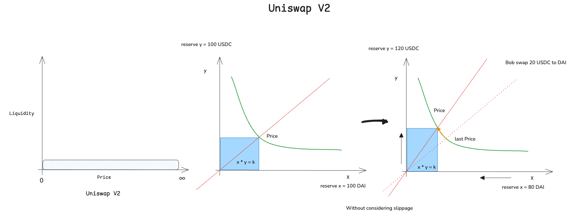
As you can see from the image, although the entire curve is supported by liquidity, one trade only moves a small path along the curve (the yellow arc on the right), which means that most of the liquidity is not used in this transaction.

So a natural question is: is it possible to provide liquidity only around this local path? This is exactly the core idea of Uniswap V3.

In V3, liquidity is no longer distributed across the entire price range, but concentrated within a limited range [p_lower, p_upper] (written as P_A and P_B in the white paper).

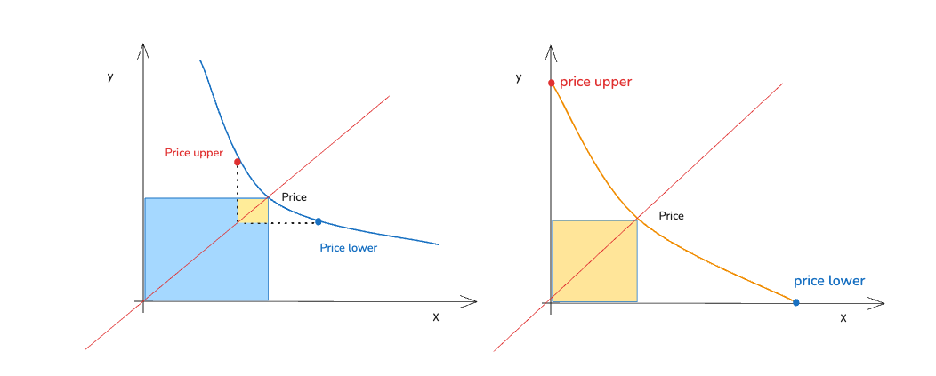
The orange area in the picture on the left represents the liquidity provided over the interval. Liquidity is no longer globally distributed, but concentrated within a limited range. If we zoom in on this orange range, we can see that in the range on the right, the price still moves along a curve similar to x * y = k. However, this curve does not exist independently; it is embedded in a larger AMM curve.

To maintain a continuous and consistent price function while providing only local liquidity, V3 introduces virtual liquidity. The core idea is to add offsets x_virtual and y_virtual in the x and y directions, embedding the current true state (x, y) into a larger coordinate system so that the state still lies on a complete AMM curve.

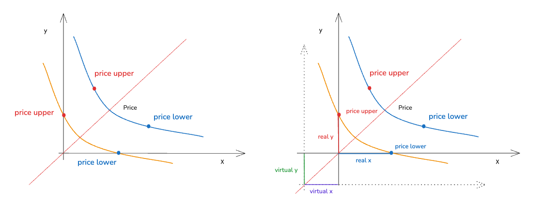
After introducing virtual liquidity, we can embed the current state into a complete constant product curve:

$$(x_R + x_V)(y_R + y_V) = L^2$$

in:

• $x_R, y_R$: real reserves
• $x_V, y_V$: virtual reserves
• $L$: liquidity